Geocoding Data - Manatee County Schools

This week's lab project introduced me to Geocoding within ArcGIS Pro and some Excel spreadsheet tactics used to prepare the data for it. The focus of this project is to extract the geographic location for Manatee County Schools from the list posted on the Florida Department of Education web site.

Started the lab with a simple copy and paste of the schools list, which includes 84 entries ranging from Charter Schools to Colleges. Added these to an Excel spreadsheet and proceeded to format the data for processing by ArcGIS Pro. The end result were data columns including the school's name, street address, city and zip code.

With the Excel spreadsheet saved as a .CSV file, proceeded into ArcGIS Pro with downloaded TIGER line shapefile data for Manatee County, Florida. The schools list data was then imported into a table.

Geocoding in ArcGIS Pro utilizes either an X/Y location using latitude/longitude, or in the case here, with an address location. First, we needed to compile an address locator file for Manatee County. Using the Create Locator tool, parameters on the TIGER line fields were set for the street name, zip codes right and left for the side of a street segment, and similarly left and right house number ranges. The process ran on the Manatee County line file, creating the Address Locator file needed for the Geocode Table tool.

The Geocode Table tool cross references the Schools input table with the Address Locator file. With our three columns of location data from the original Excel sheet, selected Address, City and Zip as the Data for the Locator Field within the tool. The process creates a geocoded point file of all school locations.

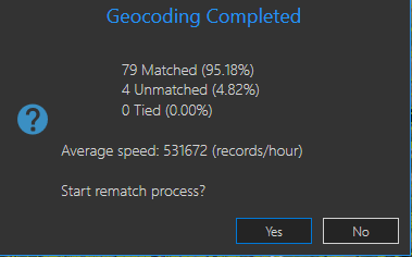
Of the 83 entries within the Schools table, all but four were matched. Those needed further analysis to be located.

One of the entries was located simply by abbreviating "Street" in the address field to "St". Based upon Florida State Road addresses, the remaining three were manually placed by researching their location.

The data entry for Carlos E. Haile Middle School used Fl 64 as the address street name. A problem with this is that often numbered routes have formal names that are used for postal addressing. Furthermore, while FL 64 implies Florida State Road 64, FDOT and other government agencies often instead use "SR" on signing and for addressing.

Two of the schools were addressed as "State Route 70" or "SR 70". The TIGER line data uses 53rd Avenue E in the FULLNAME field for the segment of SR 70 where the schools are actually located. So those schools are misplaced. Contrary to that, two of the original unmatched schools are located along SR 64 in Lakewood Ranch, which the TIGER line data references incorrectly as Manatee Avenue. Manatee Avenue is the formal name for SR 64 within Bradenton. East of there, State Road 64 is the formal name for SR 64 in unincorporated Manatee County.

Data quality is definitely a concern for when it comes to Geocoding. Whether it be an inaccurate address or missing data, these can result in potentially time consuming problems.

Published the final geoprocessed data, showing Manatee County populated with the various school locations, on the webmap at https://pns.maps.arcgis.com/home/item.html?id=c66a66146c024cec9064604c851b0f23. Edited the webmap on September 26 to show a second point layer including the geocoded school list with all locations corrected.

Buffer Analysis with Desoto National Forest data

This week's GIS Lab introduced spatial analysis and more specifically, the concept of buffers. Buffers in GIS can be applied to spatial data to conduct analysis on a specifically defined area surrounding the data in question. My last experience with buffers was back in 1998 at the University of Delaware. Our final project then used buffers as part of the analysis for the White Clay Creek Watershed in northern Delaware. Still having the paperwork from my GIS work back then, I scanned some of the maps to show buffers that we used:

Please ignore the lack of a North Arrow and Scale Bar, that was a long time ago!

The map to be produced for our Vector analysis lab will show potential campground sites within DeSoto National Forest in southeastern Mississippi. The criteria for a suitable campsite includes locations no more than 300 meters from a road, so that they are accessible by car. Sites should also be within 500 meters from a river for recreational opportunities. However sites should be at least 150 meters from a lake, to offset potential flooding concerns from larger bodies of water. Possible sites also need to exclude areas within conservation areas where plants and wildlife are protected.

Vector data acquired for this analysis includes feature classes for roads across the National Forest, hydro data including both lakes and rivers, and a polygon layer for conservation areas. GIS analysis utilizes a series of buffers on both the roads and hydro data to find areas within optimal range from roads and rivers, but a safe distance from lakes and wholly outside conservation areas.

Initial analysis utilized a fixed distance buffer including all areas within 300 meters from area roads. Dissolving the output feature class for the roads buffer resulted in one seamless polygon in place of separate abutting polygons. Followed this with a variable buffer on the hydro data. First adding a field for buffer distance (buffdist) to the attribute table, I used the Calculate Field function to set a buffdist of 500 meters for rivers and a buffdist of 150 meters for lakes. 

Next ran the Geoprocessing buffer tool with the buffdist Field as the distance parameter and Planar as the method since projected coordinate systems were used for the data. The output feature class used dissolved features based upon the buffdist Field. This produced separate polygons for areas within 150 meters of a lake and 500 meters from a river.

With feature classes for roads buffer and water buffer compiled, analysis shifted to overlaying the two. Continued by adding a new field "insd_wbuf" for inside water buffer and "insd_rbuf" for inside road buffer on the respective layers. Both fields were set to short integers, instituting a Boolean expression where 1 equals yes or is True, and 0 is no or is False. Ran the Union (Analysis) Tool on the buffers, producing a new feature class. Polygons varied from "areas within the lake buffer, but outside the road buffer" to "areas within both the river and road buffer."

The resulting layer from the Union Tool assigned areas within both the roads and water buffers as 1 (True) for the insd_wbuf and insd_rbuf fields. Selected those attributes where both fields were set to 1 and exported the features into a new feature class.

Lastly, the conservation areas were excluded from the feature class containing areas within falling within both roads and water buffers. With those areas eliminated from consideration, the final layer showing possible campground sites was nearly ready to be reviewed.

The resulting feature class was a multipart layer, meaning that while the various polygons appeared separate, they were all part of a single attribute record. The Multipart to Singlepart tool partitioned the data into single sites. One last step involved adding the field Area to the final attribute table and calculating the area of each site feature in hectares.

All geoprocessing completed, the data showing areas that fit our criteria for optimal campground locations was ready for presentation. How big is a hectare? 1 hectare is 2.47 acres. So for the symbology, I color coded areas based upon size, with larger areas represented with darker shades of green. Reading that RV parks often require 5 to 20 acres of land, I excluded all areas that were below 2 hectares.

Following a series of several revisions, the final map:

 

Map Projection Variation with Florida County data

This week's GIS lab delved into map projections, the manipulation of attribute data and the creation of a feature class out of selected data. We were tasked with taking a polygon shapefile of Florida's County Boundaries and reprojecting it from the original Albers Conical Equal Area (Albers) coordinate system to both the State Plane Coordinate System (State Plane Florida North) and the Universal Transverse Mercator (UTM 16 North) system.

Following the completion of that task, we were asked to compare the three maps to note any differences. The Albers and State Plane map projections were very similar, while the UTM projection was noticeably tilted more. Further analysis involved extracting the area in square miles in tables for four select counties across the state. When comparing them, Escambia was nearly identical in area on all three. Alachua was only four square miles larger on UTM 16 N as compared to the other two. More substantial differences were noted in Miami-Dade and Polk Counties, where the square mile numbers for UTM 16 N remained the highest.

Final map showing Florida with a selected Counties layer in Albers, FL State Plane N and UTM 16 N

Our process summary included a section to report my results and conclusions. While I knew of the concept of projections from previous cartography work, I really did not know much about the origins of their geographic coordinate systems. So I devoted several hours of research, composing a word document on them for future reference. Followed this by practicing reprojection more and creating overview maps showing each of the three projections nationally with graticules.

With an understanding of their methodology, the differences in the three Florida County map projections become more clear. The original shape file uses the Albers coordinate system, which it turns out is optimal to use for east to west geographical areas located in the mid latitudes. More specifically, the coordinate system uses a two standard parallels to minimize distortion in the region between them. This results in spatial accuracy along the parallels and minimum distortion between them. However scale along the lines of longitude does not match the scale along the lines of latitude, resulting in the final projection not being conformal. Albers is best suited for projecting the entire state of Florida.

There are 60 UTM zones per hemisphere, each spanning 6° longitude with a central meridian located around 180 kilometers between the edges. Best suited for north-south regions, the scale error does not exceed 0.1% per zone. Error and distortion increases for regions that span more than one UTM zone. A UTM zone is not designed for areas spanning more than 20 degrees of latitude.

Within this lab, Florida was projected using UTM 16 N, with a central meridian crossing the Florida Panhandle. The entire Florida Peninsula is within UTM 17N. Therefore while the scale error is still minimal, county areas are larger than with Albers or State Plane.

The State Plane Coordinate System divides the 50 U.S. states and associated U.S. territories to over 120 numbered zones. An assigned code for each zone defines the projection parameters using one of three conformal projections. The system is designed with a maximum scale distortion of one part in 10,000 per zone, with a central meridian or standard parallels maintaining this level of accuracy.

The Florida County boundaries layer projected in the lab uses Florida State Plane North, one of three zones assigned to the Sunshine State. This zone uses Lambert Conformal Conic projection, which is best for middle latitudes, as long as the range does not exceed 35°. Similar to Albers, Lambert portrays shape more accurately than area. Latitude spacing increases beyond the standard parallels, with minimal distortion near them. Scale is correct along the standard parallels, but reduced between them and increased beyond them.

The Florida Peninsula generally falls within Florida State Plane West or East. Alachua County represents the eastern extent of the North zone, so the area is accurate. Polk and Miami-Dade are located in the other zones, and therefore are scaled slightly higher due to being beyond the standard parallels for Florida State Plane North.

Florida State Plane East and West both use  Transverse Mercator projection, as they have long north to south axes.

ArcGIS Field Maps - Tampa area route markers

Three weeks into GIS4043, we were introduced to a package including data collection, ArcGIS Online, Story Maps and ArcGIS Field Maps. While I have worked with ArcGIS Online creating state maps with data from various Departments of Transportation for research and write-ups for pages on AARoads, a lot of this was new to me.

The purpose of this week's lab is to create a Feature Class with data collected with a mobile unit using ArcGIS Field Maps. Then with that data, creating a web layer to be shared online by multiple methods.

The initial steps in the lab were to create an empty project and utilize Domains. Domains are predetermined options for data collection in the field. For this project, we were to select an aspect of Public Safety, either within a building complex or in a geographical area.

Seeing the opportunity to couple the data collection with an aspect of AARoads, I chose Route Sign Markers as the Public Safety aspect to collect. The clear and consistent marking of numbered routes not only aids in motorist navigation but also indicates that a street or highway is part of a larger system maintained by either the county or state. Clearly marked routes reduce motorist confusion, allowing more attention to be devoted to driving in place of navigation. Poorly marked routes, or ones not marked at all can lead to last minute decisions as far as where to turn or frustration with taking the wrong road altogether.

Florida State Road 597 marker in excellent condition

Faded CR 582 marker in North Tampa

 

Furthermore, GPS based navigation systems such as Google Maps and TomTom devices tend to favor referencing numbered routes over named streets. Therefore having consistently signed route markers working in tandem with street names is better from a motorist perspective. Well marked routes can also aid in hurricane evacuations, keep trucks on designated routes, and provide signed alternates due to congestion on primary routes.

With that in mind, the Domain set up for this lab is "condition", with the field providing options (Code) for excellent, fair and poor. The field type was set to text, and a short description of each Code was entered. This set of criteria works out well with route sign markers, as part of my inspiration for what to collect is because FDOT similarly does field collection where every sign within a district is cataloged in the field and rated based upon its condition.

Following the Domains creation, next was the creation of a new Feature Class that will be populated with the data collected in the field. Having some knowledge of MySQL databases made understanding the need for the Data Type of "Condition" to be set as Text, so it matched the Domain field type set earlier. Other fields added included Photo with the Data Type of Raster and Notes with the Data Type of Text.

With the new Feature Class added to our project Geodatabase, I applied the Condition Domain to the Condition Field. This allows the predetermined Conditions to be used in the field. I then shared the empty Feature Class as a Web Layer with it configured to allow editing. Following a hiccup where the unique numeric ID was not preset (another aspect of MySQL coming into play), the page was published to the Content section of my ArcGIS Online account.

Added the Field Maps application to my Samsung phone via the Google Play Store. Once logged in, data collection could commence! My initial point was a test in the office of a prototype road sign made for me. With the success of that, the next point was within walking distance along U.S. 41.

For the remainder of the points, I wanted a variety of examples allowing me to categorize some signs as fair and others as poor. Knowing where several arrays of such were, my brother, who is a Professional Surveyor, accompanied me as we drove to collect nearly a dozen points. He mentioned Survey Grade collection, which is placing the collection device as close to the data to be cataloged as possible. So I went with that method, placing my phone against each sign support post for the collection.

The various route markers we collected throughout the Lutz and North Tampa area

No major difficulty with collecting the points. The only somewhat confusing aspect was that even after touching the Check button in Field Maps to finalize a data point, occasionally the data entry dialog remained. This initially led me to question whether or not the data I entered went through.

Once back at the PC, verified that the data collection was successful on the Web Map on ArcGIS Online. Opened the map via Portal in ArcGIS Pro as well, noting that the pop up information on the software omits the photo thumbnail for each point. Also created a Map Package from the map layer and KML files for Google Earth.

The finished Web Map was posted at https://pns.maps.arcgis.com/apps/mapviewer/index.html?webmap=acd601fc59ab435391f633fe99df7e66