Spatial Data Quality - Road Network Completeness

Continuing the focus on Spatial Data Quality in GIS Special Topics, Module 1.3 covers the Accuracy Assessment of Roads. Road networks are widely used as the basemap for many applications. This factors into expectations for positional accuracy and completeness, which this week's lab covers.

Road networks are also used for geocoding and network routing. The usability of such is dependent upon robust attributes such as street names, address numbers, zip codes in addition to networking aspects such as turn restrictions and one-way directions. Topologically, road networks must also be robust, with exact connectivity found in reality (Zanbergen 2004).

Typically road network datasets are compiled from an array of historical sources, with digitization from aerial imagery and augmentation from GPS field data collection. One of the most comprehensive datasets in the U.S. with a long lineage is TIGER (Topologically Integrated Geographic Encoding and Referencing).

Produced by the US Census Bureau for 1:100,000 scale maps (Syoung & O'Hara, 2009), TIGER was originally compiled to be topologically correct. That is data was not focused on being as accurate as possible, but instead data stressed connections and boundaries. (Zanbergen 2004) This resulted in legacy errors, which were carried over in succeeding updates from 2000 onward.

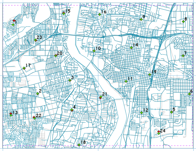
TIGER roads centerline data for Jackson County, Oregon

Covered in the last week's lab, accuracy assessment of roads utilizes methods such as "ground-truthing" using GPS or surveying equipment, comparing roads with high resolution imagery, and comparing roads to existing datasets deemed to be of higher accuracy.

Positional accuracy last week looked at the comparison of points between two datasets using root-mean-square-error (RMSE) with reference or true points. Additional methods include using buffers. This is where the true line is buffered with some distance to show discrepancies. It is also used to determine where displacements between matching features fall within an expected nominal accuracy. (Syoung & O'Hara, 2009) In other words data located in areas outside a buffer (specified tolerance) are deemed to be substantial errors.

Another method for positional accuracy is line displacement. This is where the displacement of various sections of a polyline are measured using Euclidean distance. Using matching algorithms, errors show the displacement of one road network from another. These displacements can be summarized (Zanbergen 2004), or be represented as a raster dataset to analyze vector geometry (Syoung & O'Hara, 2009).

The lab assignment for Module 1.3 conducts accuracy assessment for completeness on two datasets of street centerlines for Jackson County, Oregon. The feature classes are TIGER road data from 2000 and a Streets_Centerlines feature class compiled by Jackson County GIS.

Street Centerlines data from Jackson County, Oregon GIS

Completeness is one of the aspects cited by Haklay (2010) in accessing data quality. Completeness is the measure of the lack of data, i.e. how much data is expected versus how much data is present. Zanbergen (2004) references measuring the total length of a road network and comparing that to a reference scenario and secondly counting the number of missing elements as a count of features.

Both accuracy assessment scenarios for completeness overlay an arbitrary grid cell over compared datasets to determine the total length of count in a smaller unit. Then a comparison between two sets of roads based on a total length can be determined.

Haklay (2010) references completeness as asking the question of how comprehensive is the coverage of real-world objects. Generalizing this as a simple measure of completeness for our analysis, the dataset with the higher total length of polylines is assumed to be more complete.

Our analysis proceeds by projecting the Tiger roads data into StatePlane coordinates to match the other provided datasets. The shape length of each polyline in kilometers is calculated from feet into a new field for each road feature class. Statistics for total length of all road segments per dataset are then summarized for the initial assessment of completeness, where the dataset with more kilometers of roads is considered more complete.

The results were 10,805.82 km of roads for the County Street Centerlines feature class and 11,382.69 km for the Tiger roads feature class. With more data, the Tiger roads data is considered more complete.

Further accuracy assessment for completeness continues with a feature class of grid polygons to be used as the smaller units for comparison. Both feature classes were clipped so that all roads outside of the 297 grid cells were dropped. Geoprocessing using the Pairwise Intersect tool separates each road centerline dataset by grid. This provides a numerical summary indicating a simple factor of completeness on a smaller scale.

The collective length of Tiger road segments exceeds the County street centerline segment length in 162 of the 297 grid cells.
The collective length of County street centerline segments exceeds the Tiger road segment length in 134 of the 297 grid cells
Additionally one grid cell contained zero polylines for either centerline dataset.

Visualization of these results shows the percent difference for the length of Tiger roads centerline data as compared to the County roads centerline data. Statistics were calculated using a  mathematical formula:
% 𝑑𝑖𝑓𝑓𝑒𝑟𝑒𝑛𝑐𝑒 = (𝑡𝑜𝑡𝑎𝑙 𝑙𝑒𝑛𝑔𝑡ℎ 𝑜𝑓 𝑐𝑒𝑛𝑡𝑒𝑟𝑙𝑖𝑛𝑒𝑠 − 𝑡𝑜𝑡𝑎𝑙 𝑙𝑒𝑛𝑔𝑡ℎ 𝑜𝑓 𝑇𝐼𝐺𝐸𝑅 𝑅𝑜𝑎𝑑𝑠)/(𝑡𝑜𝑡𝑎𝑙 𝑙𝑒𝑛𝑔𝑡ℎ 𝑜𝑓 𝑐𝑒𝑛𝑡𝑒𝑟𝑙𝑖𝑛𝑒𝑠) ×100%
Completeness is aggregated where cells with more kilometers of Tiger roads than County roads appear in reds and oranges and shades of green where the collective length of County roads polylines exceeds the length of the Tiger roads data.

Map showing the geographic distribution in the differences of completeness for the two road datasets

References:

Zanbergen (2004, May). Spatial Data Management: Quality and Control. Quality of Road Networks. Vancouver Island University, Nanaimo, BC, Canada.

Suyoung & O'Hara (2009, December). International Journal of Geographical Information Science 23, 1503-1525.

Haklay (2010, August 1). Environment and Planning B: Planning and Design, 37, 682-703. 

Spatial Data Quality - Positional Accuracy of Road Networks

When viewing a map or working with geospatial data, it is generally assumed to be accurate. But this may not always be the case, and many factors can affect accuracy. Unaccounted bias may be present, data may have been digitized at a coarser scale than was required, errors present on a previous dataset used to update a new one could be carried over, etc. So how accurate is a map or geospatial data?

Since 1998, the National Standard for Spatial Data Accuracy (NSSDA) is the Federal Geographic Data Committee (FGDC) metric used for estimating the positional accuracy of points in the horizontal or vertical direction of geospatial data. Testing uses well-defined locations to compare observed or sample data to reference or true data. Reference data might be a higher accuracy dataset, such as data at a larger scale (1:24000 versus 1:250000). It may constitute high resolution digital imagery or field survey data.

The NSSDA methodology calculates the positional error using the coordinates of the reference or true points and the observed points of the dataset being tested. The positional error, or error difference, is simply the distance between the true coordinates and dataset coordinates. It uses the equation
√(x_t-x_d)² + (y_t-y_d)² where x_t and y_t are the true point / reference point coordinates and x_d and y_d are the sample point coordinate locations. The resulting error distance value is squared so that there are no negative numbers (no direction to the error).

Positional Error

The error distances for all sample points are summed. That total is averaged for the mean square error. Taking the square root of the mean square error determines the Root Mean Square Error (RMSE) statistic for the data set. The RMSE is then converted using a multiplication factor of 1.7308 for horizontal accuracy and 1.9600 for vertical accuracy. This results in the 95th percentile in map units. The confidence level means that 95% of the positions in the dataset will have an error equal to or lower than the reported accuracy value with regards to true ground position.

The second lab for Special Topics in GIS partially returns me to my previous life is a cartographer and map researcher. The subject of the lab is positional accuracy of road networks, and the data provided covers a portion of Albuquerque, New Mexico. One of the projects I worked on at Universal Map was an update for the Albuquerque wall map. Back then we routinely worked with TeleAtlas data, which at the time was a substantial improvement from TIGER data, but far below today's accuracy standards.

The lab works with two feature classes for the study area: a feature class of road centerlines compiled by the city of Albuquerque and streets data from StreetMap USA, a TeleAtlas product. 6" ortho images from 2006 covering the study area represent the reference data.

The second protocol of NDSSA is to collect test points from the data set to which the accuracy needs to be determined. For this we implement the Stratified Random Sampling Design, which while not always possible with some data, is the ideal approach:

• Data points should not be within a distance of one tenth the length of the diagonal of the study area.
• Partitioning the study area into four quadrants, each quadrant should have at least 20% of the sampling points.

Six per quadrant, the sampling of 24 test points for the Albuquerque study area

Within ArcGIS Pro I created a layout of the study area and added guides across the center horizontally and vertically. Points were selected based upon suitability of the ortho imagery, i.e. the reference data. The principle is similar to selecting control points for georeferencing, which ideally uses geometrically linear features such as T-intersections.

Using a T-intersection as the reference data for sample point #20

Large error distance for StreetMap USA sample point #1

With mutual ID numbers, sample points were digitized for both street centerline datasets in new feature classes. A point with a similarly corresponding ID number was digitized in a new reference feature class. Coordinate data for all points was generated using the Add XY Coordinates geoprocessing tool.

Tables for all three feature classes were exported into Microsoft Excel using the Table to Excel geoprocessing tool. Error distances were then calculated between each sample point and associated reference point. I did this at first with one formula, but then replicated the horizontal accuracy statistic worksheet provided in the Positional Accuracy Handbook from Minnesota Planning Land Management Information Center (LIMC) in Excel.

Horizontal Accuracy Assessment for StreetMap USA data

The calculations result in the error distance squared as compiled in the last column. These values are summed and then averaged. The RMSE is the square root of the mean square error, which multiplied by 1.7308 outputs the NSSDA horizontal accuracy.

Formal accuracy reporting per the FGDC document Geospatial Positioning Accuracy Standards Part 3: National Standard for Spatial Data Accuracy on page 3-5 and the Minnesota IT Services A Methodology for Measuring and Reporting Positional Accuracy in Spatial Data web page:

Tested 12.43 (feet) horizontal accuracy at 95% confidence level for the Albuquerque Streets data set.

Tested 401.65 (feet) horizontal accuracy at 95% confidence level for the Street Map USA data set.

Positional accuracy statements as reported in metadata:

Using the National Standard for Spatial Data Accuracy, the Albuquerque Streets data set tested to 12.43 feet horizontal accuracy at 95% confidence level.

Using the National Standard for Spatial Data Accuracy, the Street Map USA data set tested to 401.65 feet horizontal accuracy at 95% confidence level.

Spatial Data Quality - Precision and Accuracy Metrics

The first module of Special Topics in GIScience covers aspects of spatial data quality. Furthermore, the associated lab defines and contrasts the concepts of accuracy and precision in spatial data.

Quality generally represents a lack of error, where error in spatial data is the difference between a true value and an observed or predicted value. Rather than unrealistically attempting to know the exact error, an estimated error based upon sampling or another statistical approach or model can be used to ascertain this.

The lab for module 1 includes a point feature class of 50 waypoints collected with a Garmin GPSMAP 76 unit. We are first tasked with determining the precision of the waypoints. Precision is formally defined as a measure of the repeatability of a process. It is usually described in terms of how dispersed a set of repeat measurements are from the average measurement.

Precision is the variance of measurement to gauge how close data observations or collected data points are when taken for a particular phenomenon. If the same information is recorded multiple times, how close are these together? Tightly packed results correlate to a high level of precision. 

When shooting multiple points of the same object with a GPS unit, the coordinates should be consistent, if not identical. If internal calibrations are off, obstructions exist between the unit and open sky, or a simple user error take place, the recorded points could vary widely. This would equate to low precision.

Accuracy is a measure of error, or a difference between a true value and a represented value. Accuracy is the inverse of error, and perfect accuracy means no error at all. Expressing accuracy in simpler terms, it is the difference between the recorded location of an observation and the true point or reference location of said phenomena.

How close is the recorded data from the actual location of the data? Inaccuracies can be reported using many methods, such as by a mean value, frequency distribution or a threshold value. Positional accuracy can be measured in x,y, and z dimensions or any combination thereof. It is common to use metrics for horizontal spatial accuracy in two dimensions.

If data is numeric, such as the GPS points for Lab 1, the accuracy error can be expressed using a metric like the root mean square error (RMSE). Precision, on the other hand, is commonly measured using standard deviation or some other measure. The difference between the two is that accuracy is compared to a reference or true value while precision utilizes the average value derived from data collected.

Measuring accuracy for the GPS waypoints from the true point and precision from the average waypoint based upon the mean coordinates

Using the 68th percentile, the horizontal precision was 5.62 meters. The horizontal precision was 6.01 meters. The average waypoint was 1.13 meters off the recorded true waypoint.

There are additional aspects of accuracy to consider. Temporal accuracy means how accurate data is in terms of temporal representation. This is also referred to as currentness, meaning up to date. There are also scenarios where instead of using up to date information, historical records are more appropriate.

Thematic accuracy, or attribute accuracy, relates as to whether data contains the correct information to describe the properties of the specific data element. Misclassified data is an example of thematic inaccuracy.

There are scenarios where data can be precise but inaccurate, or imprecise but accurate. If the average of all collected or observed points falls within an acceptable threshold from the true point location, this data can be considered accurate, even if the point locations are widely place, and therefore imprecise. 

Conversely if a number of points are well clustered, but well away from the true point location, this data is considered precise but also inaccurate. This is also referred to as bias, which refers to a systematic error.

The second part of Lab 1 worked with a larger provided dataset of 200 collected points with X,Y coordinates. The RMSE was calculated using Microsoft Excel. A Cumulative Distribution Function was 

CDF showing the error distribution of collected point data

Rather than focusing on selected error metrics, the CDF gives a visual indication of the entire error distribution. The graph plots the frequency of observations based upon error. The 68th Percentile here was 3.18, and that matches the location of the CDF plot where the x-axis shows that the amount of error is 68% of the cumulative probability percentage.

References:

Zanbergen. Spatial Data Management: Quality and Control. Fundamentals of Spatial Data Quality. Vancouver Island University, Nanaimo, BC, Canada.

Bolstad, B., & Manson, S. (2022). GIS Fundamentals – 7th Edition. Eider Press.

Leonardo, Alex. (2024, June 10). Cumulative Distribution Function CDF. Statistics HowTo.com                    https://www.statisticshowto.com/cumulative-distribution-function-cdf/