Spatial Data Quality - Positional Accuracy of Road Networks

When viewing a map or working with geospatial data, it is generally assumed to be accurate. But this may not always be the case, and many factors can affect accuracy. Unaccounted bias may be present, data may have been digitized at a coarser scale than was required, errors present on a previous dataset used to update a new one could be carried over, etc. So how accurate is a map or geospatial data?

Since 1998, the National Standard for Spatial Data Accuracy (NSSDA) is the Federal Geographic Data Committee (FGDC) metric used for estimating the positional accuracy of points in the horizontal or vertical direction of geospatial data. Testing uses well-defined locations to compare observed or sample data to reference or true data. Reference data might be a higher accuracy dataset, such as data at a larger scale (1:24000 versus 1:250000). It may constitute high resolution digital imagery or field survey data.

The NSSDA methodology calculates the positional error using the coordinates of the reference or true points and the observed points of the dataset being tested. The positional error, or error difference, is simply the distance between the true coordinates and dataset coordinates. It uses the equation
√(x_t-x_d)² + (y_t-y_d)² where x_t and y_t are the true point / reference point coordinates and x_d and y_d are the sample point coordinate locations. The resulting error distance value is squared so that there are no negative numbers (no direction to the error).

Positional Error

The error distances for all sample points are summed. That total is averaged for the mean square error. Taking the square root of the mean square error determines the Root Mean Square Error (RMSE) statistic for the data set. The RMSE is then converted using a multiplication factor of 1.7308 for horizontal accuracy and 1.9600 for vertical accuracy. This results in the 95th percentile in map units. The confidence level means that 95% of the positions in the dataset will have an error equal to or lower than the reported accuracy value with regards to true ground position.

The second lab for Special Topics in GIS partially returns me to my previous life is a cartographer and map researcher. The subject of the lab is positional accuracy of road networks, and the data provided covers a portion of Albuquerque, New Mexico. One of the projects I worked on at Universal Map was an update for the Albuquerque wall map. Back then we routinely worked with TeleAtlas data, which at the time was a substantial improvement from TIGER data, but far below today's accuracy standards.

The lab works with two feature classes for the study area: a feature class of road centerlines compiled by the city of Albuquerque and streets data from StreetMap USA, a TeleAtlas product. 6" ortho images from 2006 covering the study area represent the reference data.

The second protocol of NDSSA is to collect test points from the data set to which the accuracy needs to be determined. For this we implement the Stratified Random Sampling Design, which while not always possible with some data, is the ideal approach:

• Data points should not be within a distance of one tenth the length of the diagonal of the study area.
• Partitioning the study area into four quadrants, each quadrant should have at least 20% of the sampling points.

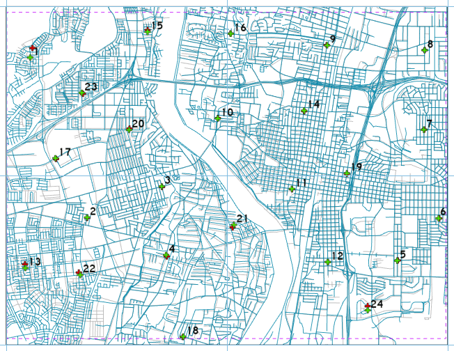
Six per quadrant, the sampling of 24 test points for the Albuquerque study area

Within ArcGIS Pro I created a layout of the study area and added guides across the center horizontally and vertically. Points were selected based upon suitability of the ortho imagery, i.e. the reference data. The principle is similar to selecting control points for georeferencing, which ideally uses geometrically linear features such as T-intersections.

Using a T-intersection as the reference data for sample point #20

Large error distance for StreetMap USA sample point #1

With mutual ID numbers, sample points were digitized for both street centerline datasets in new feature classes. A point with a similarly corresponding ID number was digitized in a new reference feature class. Coordinate data for all points was generated using the Add XY Coordinates geoprocessing tool.

Tables for all three feature classes were exported into Microsoft Excel using the Table to Excel geoprocessing tool. Error distances were then calculated between each sample point and associated reference point. I did this at first with one formula, but then replicated the horizontal accuracy statistic worksheet provided in the Positional Accuracy Handbook from Minnesota Planning Land Management Information Center (LIMC) in Excel.

Horizontal Accuracy Assessment for StreetMap USA data

The calculations result in the error distance squared as compiled in the last column. These values are summed and then averaged. The RMSE is the square root of the mean square error, which multiplied by 1.7308 outputs the NSSDA horizontal accuracy.

Formal accuracy reporting per the FGDC document Geospatial Positioning Accuracy Standards Part 3: National Standard for Spatial Data Accuracy on page 3-5 and the Minnesota IT Services A Methodology for Measuring and Reporting Positional Accuracy in Spatial Data web page:

Tested 12.43 (feet) horizontal accuracy at 95% confidence level for the Albuquerque Streets data set.

Tested 401.65 (feet) horizontal accuracy at 95% confidence level for the Street Map USA data set.

Positional accuracy statements as reported in metadata:

Using the National Standard for Spatial Data Accuracy, the Albuquerque Streets data set tested to 12.43 feet horizontal accuracy at 95% confidence level.

Using the National Standard for Spatial Data Accuracy, the Street Map USA data set tested to 401.65 feet horizontal accuracy at 95% confidence level.

Automating Geoprocessing with Python

Moving into Module 5, our assignment this week consists of writing a Python script to automate geoprocessing tasks. We were provided a dataset with several Alaska and New Mexico feature classes and the task of copying them into a newly created file geodatabase (fGDB). Working with lists and dictionaries, our script also implements several functions including ListFeatureClasses, Describe, and SearchCursor. Our end task was to output a dictionary (a Python list with pairs of keys:values) of New Mexico county seats.

As an aside, I always like working with data from places I have visited. Including an Albuquerque airport stop in 2007, I've been to New Mexico four times. I also updated the Universal Map Group Wall Map for Albuquerque as one of my projects in 2008.

I-40 west ahead of Tijeras from my trip to New Mexico in 2017.

The ListFeatureClasses() function returns a list of feature classes in the current workspace. This list can be stored in a variable to be used with subsequent functions. Part of the ArcPy package, the Describe() function returns a Describe object which includes properties of a feature class such as data type, geometry type, basename, etc.

Using the Describe function on the variable with the feature class list allows a property, such as the basename, to be used as part of the CopyFeatures() function in the Data Management toolbox. This function copies input feature class features into a new feature class. With a for loop, we used this to populate our newly created file geodatabase (fGDB) with a concatenation of a variable for the output environment, the name of our created fGDB and the basename property of each feature class.

The program flowchart for this week's Lab assignment

While the term cursor to me references the blinking vertical line in this word processor, it has a separate meaning in computer programming. Cursor is a database technology term for accessing a set of records in a table. Records in a table are referred to as rows. Iterating over the row of a table, the three cursors in Python are as follows:

• Search Cursor - this function retrieves specific rows on the basis of attribute values. This is similar to performing a SQL query.
• Insert Cursor - this function adds new roads to a table, which can in turn be populated with new attribute values.
• Update Cursor - this function modifies the attribute data of existing rows or deletes rows from the table.

Each type of cursor is created by corresponding class of the arcpy.da.module. The cursor object accessed row objects, returning a tuple of field values in an order specified by the field names argument of the function. The cursor iterates over all table rows but using only specific fields as needed.

Cursors support with statements, which have the advantage of executing regardless of whether the cursor finished running successfully and completing without a data lock. A data lock ensues otherwise is a cursor is not deleted with a del statement. The data lock prevents multiple processes from changing the same table simultaneously.

With statements also incorporate SQL queries as the where_clause optional parameter in the SearchCursor syntax. SQL queries find records in a database table based upon specific criteria selecting data WHERE specific conditions occur. I often use SQL queries when updating the database for the main AARoads pages and also occasionally with the Simple Machines Forum database on the site.

The Lab assignment specified using the SearchCursor on the feature class of point data for cities in the state of New Mexico. The search criteria fields were the city NAME, the city FEATURE type and the 2000 Census population data (POP_2000). I found that assigning the SearchCursor output as variables made formatting the print statement vastly easier and cleaner looking codewise.

The biggest challenge I had was populating the dictionary with the county seats. I eventually incorporated the process in the for loop of the SearchCursor with statement. Used the W3Schools web site to narrow down the code to use, and with the previous variables, creating the dictionary was simple.

Looking at the example output included in the Lab assignment PDF, I opted to expand upon the formatting. Being the county collector that I am, I incorporated the COUNTY name field so that the output listed the associated county with each seat. Furthermore after discovering that three of the entries lacked population data, I implemented an if statement. The missing data values showed -99999. Being that it was an integer, I first cast that as a string, and then reassigned the population variable to read "not available".

Collage of screen shots showing the output of the Module 5 Python Script