Interpolation Methods - Tampa Bay Water Quality

There are numerous spatial interpolation methods used to generate surfaces in GIS. This is the prediction of variables at unmeasured locations based upon sampling of similar variables at known locations or true points. Related, spatial prediction is the estimation of variables at unsampled locations based partly on other variables and a collective set of measurements. Comprised of spatially continuous data, surfaces could be topographic, a measure of air pollution, soil moisture, air temperatures and population density among others (Bolstad & Manson, 2022).

A number of factors can affect the performance of spatial interpolation methods. Some of these factors are data accuracy, temporality of the data, sampling design, sample spatial distribution, the presence of abnormal values or outliers, and the correlation of primary and secondary variables (Hu, 1995, Li & Heap, 2014).

Deciding upon the best interpolation method is not always a straight forward process. Methods often work well for a specific data set because of inherent assumptions and algorithm design for estimation. Different interpolations methods applied to the same data set may produce desired results for one study objective but not another (Hu, 1995).

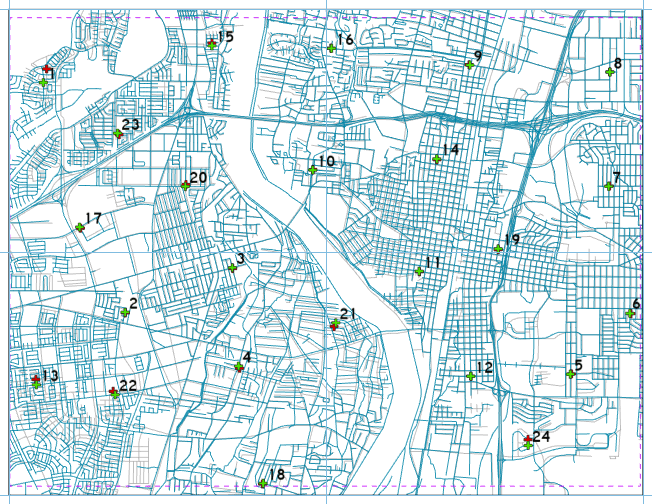
Module 5 for GIS Special Topics performs interpolation analyses for Tampa Bay water quality data. Specifically four methods are used for the estimation of Biochemical Oxygen Demand (BOD) in milligrams per liter variables for Tampa Bay. A point feature class of BOD sample locations is provided and the study area is all of Tampa Bay, Old Tampa Bay and Hillsborough Bay. A statistical analysis of each is compared in an effort to determine which derived surface best describes water quality.

The first interpolation method implemented for the Tampa Bay water quality analysis is Thiessen Polygon. This method was the easiest to interpret. It aggregates the point dataset within the study area to polygons with one per point, which is referred to as a centroid. All estimated points within the Thiessen polygon (proximal zone) are closer in value to the associated centroid than any other centroid in the overall analysis.

The Thiessen Polygon method is optimal when there is no uniform distribution of the sample points. The method is applicable to environmental management (Wrublack et. al, 2013).

The Thiessen Polygon raster with an output cell size of 250.

Previously discussed in the Isarithmic Mapping lab in Computer Cartography, the Inverse Distance Weighting (IDW) spatial interpolation method estimates values using the values of sample points and the distance to nearby known points (Bolstad & Manson, 2022). Values closer to a location have more weight on the predicted value than those further away. The power parameter in the mathematical equation of the method determines the weighting, which decreases as the distance increases. When the power parameter increases, a heavier weight is applied to nearby samples, which increases their influence on estimation (Ikechukwu, 2017).

The IDW method assumes that the underlying surface is smooth. It works well with regularly spaced data, but cannot account for the spatial clustering of sample points (Li & Heap, 2014).

The IDW raster for water quality. The power parameter was 2 and output cell size of 250.

Spline interpolation uses a mathematical function to interpolate a smooth curve along a set of sample data points with minimal curvature. Polynomial functions calculate the segments between join points. These accommodate local adjustments and define the amount of smoothing. The method is named after splines, the flexible ruler cartographers used to fit smooth curves through fixed points (Ikechukwu, 2017).

The performance of Splines improves when dense, regularly-spaced data is used (Li & Heap, 2014). The method is very suitable for estimating densely sampled heights and climatic variables (Ikechukwu, 2017).

The lab uses the options of Regularized and Tension for the Spline geoprocessing tool in ArcGIS Pro. This changes the weight parameter, where higher values in Regularized splines result in smoother surfaces. A weight of zero for the Tension spline option results in a basic thin plate spline interpolation. This is also referenced as the basic minimum curvature technique.

Estimated Tampa Bay water quality - Regularized Spline Interpolation Method

Estimated Tampa Bay water quality - Tension Spline Interpolation Method

References:

Bolstad, B., & Manson, S. (2022). GIS Fundamentals – 7th Edition. Eider Press.

Hu, J. (1995, May). Methods of generating surfaces in environmental GIS applications. In 1995 ESRI user conference proceedings.

Li, J., & Heap, A. D. (2014). Spatial interpolation methods applied in the environmental sciences: A review. Environmental Modelling & Software, 53, 173-189.

Wrublack, S. C., Mercante, E., & Vilas Boas, M. A. (2013). Water quality parameters associated with soil use and occupation features by Thiessen polygons. Journal of Food, Agriculture & Environment, 11(2), 846-853.

Ikechukwu, M. , Ebinne, E. , Idorenyin, U. and Raphael, N. (2017) Accuracy Assessment and Comparative Analysis of IDW, Spline and Kriging in Spatial Interpolation of Landform (Topography): An Experimental Study. Journal of Geographic Information System, 9, 354-371. doi: 10.4236/jgis.2017.93022.

Searching for the right GIS job

Finally got started with my GIS Internship with the Florida Department of Transportation at District 7 (D7) Headquarters last week. The position affords me the opportunity to work on several GIS related tasks and with multiple departments. I am working with a great team and providing assistance to others with ArcGIS Pro.

Settling into my internship position at D7 went very smoothly. My initial task is working on a basic training manual for ArcGIS Pro to be used in future courses that the GIS department will offer employees. Additionally I was invited to join planning meetings for this year's GIS Day, which will include demonstrations and information on how various departments across D7 use GIS. I am excited to contribute ideas and provide input, and this will also aid in my eventual GIS Day assignment for GIS4944!

One of the assignments for this week in GIS4944 is to conduct a job search for what we could consider to be our Dream GIS Job. Working on road map production for a major mapping company in GIS would be it, but the paper map industry is minimal and becoming more niche. So my second GIS job choice is working in transportation. My positive experiences after two days at FDOT have already reinforced this! 

The job that is most appealing in my search is for a GIS Analyst I for the Texas Department of Transportation (TxDOT). Generally all of the essential duties listed in the job posting fall somewhere within my knowledge wheelhouse. Collecting, preparing and digitizing GIS data is the first listed. Create, maintain, update GIS databases and cartographic products is another duty. Extraction of features from georeferenced scanner paper maps is a third duty that I have experience with. Even the bullet point referencing converting CAD and other formats into ArcGIS formats is a task I likely could master, given previous work with CAD at Mapsource and Adobe Illustrator for AARoads.

The position requires no prior experience, but a Bachelor's Degree in Geography, GIS or a related field is. However, the posting reveals that relevant work experience may be substituted for a degree on a year per year basis. I am confidence I can meet this requirement through my previous work with Mapsource, Universal Map Group, and GIS Cartography & Publishing Services, in addition to our coursework in the UWF GIS Certificate program.

The results of the GIS job search gave me a framework for what to look for in future job searches. The TxDOT position is about as optimum as I could get for both my skillset and interests. A job description for a GIS analyst position with FDOT would likely be similar. However, with ongoing budgetary issues, no positions at FDOT will be posted in the near future. There's always the private sector to consider as well.

3D Mapping - TINs and DEMs

Moving on from Spatial Data Quality in GIS Special Topics, the next Lab focuses on surfaces with a comparison of the Digital Elevation Model (DEM) and Triangular Irregular Network (TIN). A surface in GIS is a geographic phenomena represented as continuous data. Continuous spatial data references geographic objects characterized by very gradual boundaries such as temperature or elevation.

The most common way to represent elevation data is with contour lines. Contour lines are 2-dimensional features with attributes containing the value of the surface at a given location. They can be derived by the TIN vector model or the DEM raster model.

TINs are used exclusively to represent a 3-dimensional surface. A series of linked irregular triangles comprised from elevation points (nodes) in 3D (X,Y,Z) coordinates (Manandhar, 2005) occurring at any given location represent the 3D surface. The topological relationship of the network of triangles creates a continuous surface. The normal vector of each triangle is used to assign the properties of Slope and Aspect.

 

DEMs are the simplest way to represent a topographic surface. A DEM is a regular raster that uses a regular rectangular grid method (Manandhar, 2005) with cell values representing elevation or spot height. The cell size of a DEM determines the resolution. Therefore a DEM with a high number of smaller sized cells provides more accuracy than a DEM with less larger sized cells. Data becomes more implicit with larger cell sizes.

One part of this week's lab utilizes a DEM to develop a 3-dimensional Ski Run Suitability Map. Initially the supplied DEM was converted to a TIN for the 3D component for the Local Scene. The suitability parameters included Elevation where areas exceeding 2,500 meters are most favorable, Slope where angles between 30 and 45 degrees rank highest, and Aspect where south and west facing slopes are most preferred.

Following reclassification, respective rasters were generated from the DEM using geoprocessing tools in ArcGIS Pro. These in turn were input into the Weighted Overlay tool where the suitability rate for aspect is 25%, elevation is 40% and slope is 35%.

The output Ski Run Suitability Map. Lighting enhancements include shadowing and adjustment of the sun angle. The Vertical Exaggeration is 2.50.

The next part of the lab further explores TINs with adjustments to symbology between elevation, slope and aspect. The deliverable included the generation of contours and selecting appropriate colors.

Cividis color TIN with 50 meter contours and 250 meter index contours.

The last section of the lab provides a point feature class that will represent the mass points for a TIN. Geoprocessing of these points were input along with a study area soft clip polygon boundary in the Create TIN tool. The resulting TIN was modified symbolically to show contours set at an interval of 100 meters.

The same mass points feature class was input into the Spline tool to create a DEM. Contours were subsequently generated from the DEM with additional geoprocessing. The two contour feature classes were then compared.

While not necessarily more accurate, the DEM based contours have smoother curvature resulting from the implicit data values from each grid cell (Manandhar, 2005). Appearing more jagged in areas with less slope, the TIN based contours are derived from every node, where 3D coordinates are more explicit. There are less Faces (triangles) in flatter areas.

References:

Manandhar, N. (2005). Comparison of TIN and Grid Method of Contour Generation from Spot Height. Nepalese Journal on Geoinformatics, 4, 1-8.

https://www.nepjol.info/index.php/NJG/article/view/51271/38351

Spatial Data Quality - Road Network Completeness

Continuing the focus on Spatial Data Quality in GIS Special Topics, Module 1.3 covers the Accuracy Assessment of Roads. Road networks are widely used as the basemap for many applications. This factors into expectations for positional accuracy and completeness, which this week's lab covers.

Road networks are also used for geocoding and network routing. The usability of such is dependent upon robust attributes such as street names, address numbers, zip codes in addition to networking aspects such as turn restrictions and one-way directions. Topologically, road networks must also be robust, with exact connectivity found in reality (Zanbergen 2004).

Typically road network datasets are compiled from an array of historical sources, with digitization from aerial imagery and augmentation from GPS field data collection. One of the most comprehensive datasets in the U.S. with a long lineage is TIGER (Topologically Integrated Geographic Encoding and Referencing).

Produced by the US Census Bureau for 1:100,000 scale maps (Syoung & O'Hara, 2009), TIGER was originally compiled to be topologically correct. That is data was not focused on being as accurate as possible, but instead data stressed connections and boundaries. (Zanbergen 2004) This resulted in legacy errors, which were carried over in succeeding updates from 2000 onward.

TIGER roads centerline data for Jackson County, Oregon

Covered in the last week's lab, accuracy assessment of roads utilizes methods such as "ground-truthing" using GPS or surveying equipment, comparing roads with high resolution imagery, and comparing roads to existing datasets deemed to be of higher accuracy.

Positional accuracy last week looked at the comparison of points between two datasets using root-mean-square-error (RMSE) with reference or true points. Additional methods include using buffers. This is where the true line is buffered with some distance to show discrepancies. It is also used to determine where displacements between matching features fall within an expected nominal accuracy. (Syoung & O'Hara, 2009) In other words data located in areas outside a buffer (specified tolerance) are deemed to be substantial errors.

Another method for positional accuracy is line displacement. This is where the displacement of various sections of a polyline are measured using Euclidean distance. Using matching algorithms, errors show the displacement of one road network from another. These displacements can be summarized (Zanbergen 2004), or be represented as a raster dataset to analyze vector geometry (Syoung & O'Hara, 2009).

The lab assignment for Module 1.3 conducts accuracy assessment for completeness on two datasets of street centerlines for Jackson County, Oregon. The feature classes are TIGER road data from 2000 and a Streets_Centerlines feature class compiled by Jackson County GIS.

Street Centerlines data from Jackson County, Oregon GIS

Completeness is one of the aspects cited by Haklay (2010) in accessing data quality. Completeness is the measure of the lack of data, i.e. how much data is expected versus how much data is present. Zanbergen (2004) references measuring the total length of a road network and comparing that to a reference scenario and secondly counting the number of missing elements as a count of features.

Both accuracy assessment scenarios for completeness overlay an arbitrary grid cell over compared datasets to determine the total length of count in a smaller unit. Then a comparison between two sets of roads based on a total length can be determined.

Haklay (2010) references completeness as asking the question of how comprehensive is the coverage of real-world objects. Generalizing this as a simple measure of completeness for our analysis, the dataset with the higher total length of polylines is assumed to be more complete.

Our analysis proceeds by projecting the Tiger roads data into StatePlane coordinates to match the other provided datasets. The shape length of each polyline in kilometers is calculated from feet into a new field for each road feature class. Statistics for total length of all road segments per dataset are then summarized for the initial assessment of completeness, where the dataset with more kilometers of roads is considered more complete.

The results were 10,805.82 km of roads for the County Street Centerlines feature class and 11,382.69 km for the Tiger roads feature class. With more data, the Tiger roads data is considered more complete.

Further accuracy assessment for completeness continues with a feature class of grid polygons to be used as the smaller units for comparison. Both feature classes were clipped so that all roads outside of the 297 grid cells were dropped. Geoprocessing using the Pairwise Intersect tool separates each road centerline dataset by grid. This provides a numerical summary indicating a simple factor of completeness on a smaller scale.

The collective length of Tiger road segments exceeds the County street centerline segment length in 162 of the 297 grid cells.
The collective length of County street centerline segments exceeds the Tiger road segment length in 134 of the 297 grid cells
Additionally one grid cell contained zero polylines for either centerline dataset.

Visualization of these results shows the percent difference for the length of Tiger roads centerline data as compared to the County roads centerline data. Statistics were calculated using a  mathematical formula:
% 𝑑𝑖𝑓𝑓𝑒𝑟𝑒𝑛𝑐𝑒 = (𝑡𝑜𝑡𝑎𝑙 𝑙𝑒𝑛𝑔𝑡ℎ 𝑜𝑓 𝑐𝑒𝑛𝑡𝑒𝑟𝑙𝑖𝑛𝑒𝑠 − 𝑡𝑜𝑡𝑎𝑙 𝑙𝑒𝑛𝑔𝑡ℎ 𝑜𝑓 𝑇𝐼𝐺𝐸𝑅 𝑅𝑜𝑎𝑑𝑠)/(𝑡𝑜𝑡𝑎𝑙 𝑙𝑒𝑛𝑔𝑡ℎ 𝑜𝑓 𝑐𝑒𝑛𝑡𝑒𝑟𝑙𝑖𝑛𝑒𝑠) ×100%
Completeness is aggregated where cells with more kilometers of Tiger roads than County roads appear in reds and oranges and shades of green where the collective length of County roads polylines exceeds the length of the Tiger roads data.

Map showing the geographic distribution in the differences of completeness for the two road datasets

References:

Zanbergen (2004, May). Spatial Data Management: Quality and Control. Quality of Road Networks. Vancouver Island University, Nanaimo, BC, Canada.

Suyoung & O'Hara (2009, December). International Journal of Geographical Information Science 23, 1503-1525.

Haklay (2010, August 1). Environment and Planning B: Planning and Design, 37, 682-703. 

GIS Internship - Networking in Tampa

The GIS Internship part of the UWF GIS Certification program is something I have looked forward to since the start of classes last Fall. While working on AARoads is rewarding, the lack of a team to work with, especially in recent years, has been increasingly discouraging. Also my previous work with GIS Cartography and Publishing Services (GISCAPS) is 100% remote, so the interaction there is limited to phone calls. Being able to work with others again and contribute to something meaningful was part of my motivation for returning to college.

Over the years I have gotten know several of the folks working at the Florida Department of Transportation District 7 here in Tampa. Ideally I wanted to work with FDOT as my internship. Unfortunately budget concerns precluded the department from offering a formal internship opportunity. However, the window of opportunity did not fully close with District 7, as thanks to research efforts from my brother in Survey and Mapping, it turns out FDOT does have a formal Volunteer Program.

The objectives of the Volunteer Program "is to enhance the delivery of quality services by promoting community involvement in the Department of Transportation, while providing volunteers with a chance to contribute their valuable time and talents." Compensation was not my goal for an internship, instead I  sought the opportunity to further enhance and expand my GIS skillset. While there were some paperwork issues to address and HR related aspects to iron out, I was approved for the Volunteer Program on August 26!

With my cartography background spanning two decades, I will be provided the opportunity to help out multiple departments at FDOT. Some of my duties outlined for the GIS Volunteer program include learning how to create map services, web maps and web applications, reviewing and providing recommendations for symbology settings for GIS layers, and helping draft a training manual for making maps in ArcGIS Pro according to D7 specifications. I will also get to work with the Survey and Mapping department.

This Fall I also registered to attend the GeoFlo Summit, which takes place on November 14, 2024 in Plant City. This will be the second time I have attended the meeting of GIS Users, but first time as an active GIS User! One of the sponsors of the event is the Tampa Bay GIS Users Group (TBGIS). TBGIS regularly hosts Networking Socials, and the next one takes place this evening in Seminole Heights, Tampa. There is no formal membership to TBGIS and everyone in the GIS community and anyone curious about the geospatial world is welcomed to join any of their events. Social media connections and where to join the TBGIS mailing list is at TBGIS Updates.

Thanks to my work with GISCAPS, I was able to attend the ESRI User Conference in San Diego back in 2014. I also attended the FDOT Symposium in 2019. Those were large-scale events, but the premise was the same, being able to meet with and interact with others in the GIS industry. I chose to focus on  TBGIS because they are local and offer in-person events.

Spatial Data Quality - Positional Accuracy of Road Networks

When viewing a map or working with geospatial data, it is generally assumed to be accurate. But this may not always be the case, and many factors can affect accuracy. Unaccounted bias may be present, data may have been digitized at a coarser scale than was required, errors present on a previous dataset used to update a new one could be carried over, etc. So how accurate is a map or geospatial data?

Since 1998, the National Standard for Spatial Data Accuracy (NSSDA) is the Federal Geographic Data Committee (FGDC) metric used for estimating the positional accuracy of points in the horizontal or vertical direction of geospatial data. Testing uses well-defined locations to compare observed or sample data to reference or true data. Reference data might be a higher accuracy dataset, such as data at a larger scale (1:24000 versus 1:250000). It may constitute high resolution digital imagery or field survey data.

The NSSDA methodology calculates the positional error using the coordinates of the reference or true points and the observed points of the dataset being tested. The positional error, or error difference, is simply the distance between the true coordinates and dataset coordinates. It uses the equation
√(x_t-x_d)² + (y_t-y_d)² where x_t and y_t are the true point / reference point coordinates and x_d and y_d are the sample point coordinate locations. The resulting error distance value is squared so that there are no negative numbers (no direction to the error).

Positional Error

The error distances for all sample points are summed. That total is averaged for the mean square error. Taking the square root of the mean square error determines the Root Mean Square Error (RMSE) statistic for the data set. The RMSE is then converted using a multiplication factor of 1.7308 for horizontal accuracy and 1.9600 for vertical accuracy. This results in the 95th percentile in map units. The confidence level means that 95% of the positions in the dataset will have an error equal to or lower than the reported accuracy value with regards to true ground position.

The second lab for Special Topics in GIS partially returns me to my previous life is a cartographer and map researcher. The subject of the lab is positional accuracy of road networks, and the data provided covers a portion of Albuquerque, New Mexico. One of the projects I worked on at Universal Map was an update for the Albuquerque wall map. Back then we routinely worked with TeleAtlas data, which at the time was a substantial improvement from TIGER data, but far below today's accuracy standards.

The lab works with two feature classes for the study area: a feature class of road centerlines compiled by the city of Albuquerque and streets data from StreetMap USA, a TeleAtlas product. 6" ortho images from 2006 covering the study area represent the reference data.

The second protocol of NDSSA is to collect test points from the data set to which the accuracy needs to be determined. For this we implement the Stratified Random Sampling Design, which while not always possible with some data, is the ideal approach:

• Data points should not be within a distance of one tenth the length of the diagonal of the study area.
• Partitioning the study area into four quadrants, each quadrant should have at least 20% of the sampling points.

Six per quadrant, the sampling of 24 test points for the Albuquerque study area

Within ArcGIS Pro I created a layout of the study area and added guides across the center horizontally and vertically. Points were selected based upon suitability of the ortho imagery, i.e. the reference data. The principle is similar to selecting control points for georeferencing, which ideally uses geometrically linear features such as T-intersections.

Using a T-intersection as the reference data for sample point #20

Large error distance for StreetMap USA sample point #1

With mutual ID numbers, sample points were digitized for both street centerline datasets in new feature classes. A point with a similarly corresponding ID number was digitized in a new reference feature class. Coordinate data for all points was generated using the Add XY Coordinates geoprocessing tool.

Tables for all three feature classes were exported into Microsoft Excel using the Table to Excel geoprocessing tool. Error distances were then calculated between each sample point and associated reference point. I did this at first with one formula, but then replicated the horizontal accuracy statistic worksheet provided in the Positional Accuracy Handbook from Minnesota Planning Land Management Information Center (LIMC) in Excel.

Horizontal Accuracy Assessment for StreetMap USA data

The calculations result in the error distance squared as compiled in the last column. These values are summed and then averaged. The RMSE is the square root of the mean square error, which multiplied by 1.7308 outputs the NSSDA horizontal accuracy.

Formal accuracy reporting per the FGDC document Geospatial Positioning Accuracy Standards Part 3: National Standard for Spatial Data Accuracy on page 3-5 and the Minnesota IT Services A Methodology for Measuring and Reporting Positional Accuracy in Spatial Data web page:

Tested 12.43 (feet) horizontal accuracy at 95% confidence level for the Albuquerque Streets data set.

Tested 401.65 (feet) horizontal accuracy at 95% confidence level for the Street Map USA data set.

Positional accuracy statements as reported in metadata:

Using the National Standard for Spatial Data Accuracy, the Albuquerque Streets data set tested to 12.43 feet horizontal accuracy at 95% confidence level.

Using the National Standard for Spatial Data Accuracy, the Street Map USA data set tested to 401.65 feet horizontal accuracy at 95% confidence level.

Spatial Data Quality - Precision and Accuracy Metrics

The first module of Special Topics in GIScience covers aspects of spatial data quality. Furthermore, the associated lab defines and contrasts the concepts of accuracy and precision in spatial data.

Quality generally represents a lack of error, where error in spatial data is the difference between a true value and an observed or predicted value. Rather than unrealistically attempting to know the exact error, an estimated error based upon sampling or another statistical approach or model can be used to ascertain this.

The lab for module 1 includes a point feature class of 50 waypoints collected with a Garmin GPSMAP 76 unit. We are first tasked with determining the precision of the waypoints. Precision is formally defined as a measure of the repeatability of a process. It is usually described in terms of how dispersed a set of repeat measurements are from the average measurement.

Precision is the variance of measurement to gauge how close data observations or collected data points are when taken for a particular phenomenon. If the same information is recorded multiple times, how close are these together? Tightly packed results correlate to a high level of precision. 

When shooting multiple points of the same object with a GPS unit, the coordinates should be consistent, if not identical. If internal calibrations are off, obstructions exist between the unit and open sky, or a simple user error take place, the recorded points could vary widely. This would equate to low precision.

Accuracy is a measure of error, or a difference between a true value and a represented value. Accuracy is the inverse of error, and perfect accuracy means no error at all. Expressing accuracy in simpler terms, it is the difference between the recorded location of an observation and the true point or reference location of said phenomena.

How close is the recorded data from the actual location of the data? Inaccuracies can be reported using many methods, such as by a mean value, frequency distribution or a threshold value. Positional accuracy can be measured in x,y, and z dimensions or any combination thereof. It is common to use metrics for horizontal spatial accuracy in two dimensions.

If data is numeric, such as the GPS points for Lab 1, the accuracy error can be expressed using a metric like the root mean square error (RMSE). Precision, on the other hand, is commonly measured using standard deviation or some other measure. The difference between the two is that accuracy is compared to a reference or true value while precision utilizes the average value derived from data collected.

Measuring accuracy for the GPS waypoints from the true point and precision from the average waypoint based upon the mean coordinates

Using the 68th percentile, the horizontal precision was 5.62 meters. The horizontal precision was 6.01 meters. The average waypoint was 1.13 meters off the recorded true waypoint.

There are additional aspects of accuracy to consider. Temporal accuracy means how accurate data is in terms of temporal representation. This is also referred to as currentness, meaning up to date. There are also scenarios where instead of using up to date information, historical records are more appropriate.

Thematic accuracy, or attribute accuracy, relates as to whether data contains the correct information to describe the properties of the specific data element. Misclassified data is an example of thematic inaccuracy.

There are scenarios where data can be precise but inaccurate, or imprecise but accurate. If the average of all collected or observed points falls within an acceptable threshold from the true point location, this data can be considered accurate, even if the point locations are widely place, and therefore imprecise. 

Conversely if a number of points are well clustered, but well away from the true point location, this data is considered precise but also inaccurate. This is also referred to as bias, which refers to a systematic error.

The second part of Lab 1 worked with a larger provided dataset of 200 collected points with X,Y coordinates. The RMSE was calculated using Microsoft Excel. A Cumulative Distribution Function was 

CDF showing the error distribution of collected point data

Rather than focusing on selected error metrics, the CDF gives a visual indication of the entire error distribution. The graph plots the frequency of observations based upon error. The 68th Percentile here was 3.18, and that matches the location of the CDF plot where the x-axis shows that the amount of error is 68% of the cumulative probability percentage.

References:

Zanbergen. Spatial Data Management: Quality and Control. Fundamentals of Spatial Data Quality. Vancouver Island University, Nanaimo, BC, Canada.

Bolstad, B., & Manson, S. (2022). GIS Fundamentals – 7th Edition. Eider Press.

Leonardo, Alex. (2024, June 10). Cumulative Distribution Function CDF. Statistics HowTo.com                    https://www.statisticshowto.com/cumulative-distribution-function-cdf/