Suitability Modeling with GIS

Module 6 for GIS Applications includes four scenarios conducting Suitability and Least-Cost Path and Corridor analysis. Suitability Modeling identifies the most suitable locations based upon a set of criteria. Corridor analysis compiles an array of all the least-cost paths solutions from a single source to all cells within a study area.

For a given scenario, suitability modeling commences with identifying criteria that defines the most suitable locations. Parameters specifying such criteria could include aspects such as percent grade, distance from roads or schools, elevation, etc.

Each criteria next needs to be translated into a map, such as a DEM for elevation. Maps for each criteria are then combined in a meaningful way. Often Boolean logic is applied to criteria maps where suitability is assigned the value of true and non suitable is false. Boolean suitability modeling overlays maps for all criteria and then determines where all criterion is met. The result is a map showing areas suitable versus not suitable.

Another evaluation system in suitability modeling use Scores or Ratings. This scenario expresses criterion as a map showing a range of values from very low suitability to very high, with intervening values in between. Suitability is expressed as a dimensionless score, often by using Map Algebra on associated rasters.

Scenario 1 for lab 6 analyzes a study area in Jackson County, Oregon for the establishment of a conservation area for mountain lions. Four sets of criterion area are specified. Suitable areas must have slopes exceeding 9 degrees, be covered by forest, be located within 2,500 feet of a river and more than 2,500 feet from highways. 

Flowchart outlining input data and geoprocessing steps.

Working with a raster of landcover, a DEM and polyline feature classes for rivers and highways, we implement Boolean Suitability modeling in Vector. The DEM raster is converted to a slope raster, so that it can be reclassified into a Boolean raster where slopes above 9 feet are assigned the value of 1 (true) and those below 0 (false). The landcover raster is simply reclassified where cells assigned to the forest land use class are true in the Boolean.

Buffers were created on the river and highway feature classes, where areas within 2,500 feet of the river are true for suitability and areas within 2,500 feet of the highway are false for suitability. Once the respective rasters are converted to polygons and the buffer feature classes clipped to the study area, a criteria union is generated using geoprocessing. The suitability is deduced based upon the Boolean values of that feature class and selected by a SQL query to output the final suitability selection.

We repeat this process, but utilizing Boolean Suitability in Raster. Using the Euclidean Distance tool in ArcGIS Pro, buffers for the river and highway feature classes were output as raster files where suitability is assigned the value of 1 for true and 0 for false. Utilized the previously created Boolean rasters for slope and landcover.

Obtaining the suitable selection raster with the four rasters utilizes the Raster Calculator geoprocessing tool. Since the value of 1 is true for suitability in the four rasters, simply adding the cell values for all result in a range of 0 to 4, where 4 equates to fully suitable. The final output was a Boolean where 4 was reclassified as 1 and all other values were assigned NODATA.

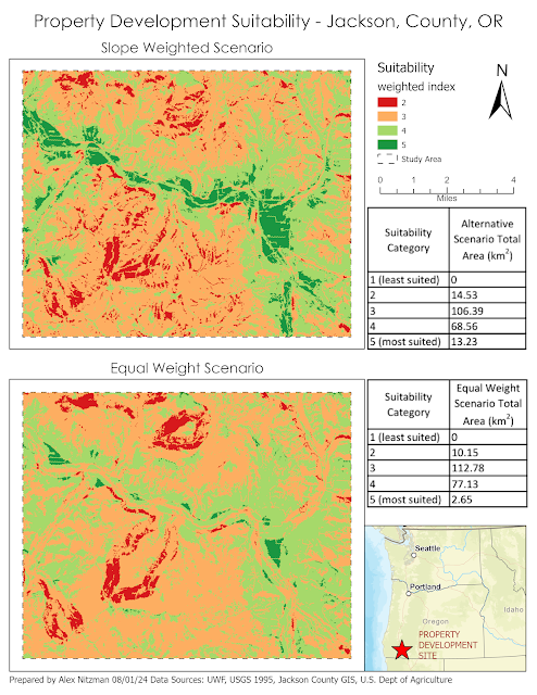
Scenario 2 determines the percentage of a land area suitable for development in Jackson County, Oregon. The suitability criteria ranks land areas comprising meadows or agricultural areas as most optimal. Additional criterion includes soil type, slopes of less than 2 degrees, a 1,000 foot buffer from waterways and a location within 1,320 feet of existing roads. Input datasets consist of rasters for elevation and landcover, and feature classes for rivers, roads and soils.

Flowchart of the geoprocessing for Scenario 2

With all five criteria translated into respective maps, we proceed with combining them into a final result. However with Scenario 2, the Weighted Overlay geoprocessing tool is implemented. This tool utilizes a percentage influence on each input raster corresponding to the raster's significance to the criterion. The percentages of each raster input must total 100 and all rasters must be integer-based.

Cell values of each raster are multiplied by their percentage influence and the results compiled in the generation of an output raster. The first scenario evaluated for lab 6 includes an equal weight scenario, where the 5 raster files have the same percentage influence (20%). The second scenario assigned heavier weight to slope (40%) while retaining 20% influence to land cover and soils criterion, and decreasing the percentage influence of road and river criterion to 10%. The final comparison between the two scenarios:

Opted to symbolize the output rasters using a diverging color scheme from ColorBrewer.