GIS Internship - Networking in Tampa

The GIS Internship part of the UWF GIS Certification program is something I have looked forward to since the start of classes last Fall. While working on AARoads is rewarding, the lack of a team to work with, especially in recent years, has been increasingly discouraging. Also my previous work with GIS Cartography and Publishing Services (GISCAPS) is 100% remote, so the interaction there is limited to phone calls. Being able to work with others again and contribute to something meaningful was part of my motivation for returning to college.

Over the years I have gotten know several of the folks working at the Florida Department of Transportation District 7 here in Tampa. Ideally I wanted to work with FDOT as my internship. Unfortunately budget concerns precluded the department from offering a formal internship opportunity. However, the window of opportunity did not fully close with District 7, as thanks to research efforts from my brother in Survey and Mapping, it turns out FDOT does have a formal Volunteer Program.

The objectives of the Volunteer Program "is to enhance the delivery of quality services by promoting community involvement in the Department of Transportation, while providing volunteers with a chance to contribute their valuable time and talents." Compensation was not my goal for an internship, instead I  sought the opportunity to further enhance and expand my GIS skillset. While there were some paperwork issues to address and HR related aspects to iron out, I was approved for the Volunteer Program on August 26!

With my cartography background spanning two decades, I will be provided the opportunity to help out multiple departments at FDOT. Some of my duties outlined for the GIS Volunteer program include learning how to create map services, web maps and web applications, reviewing and providing recommendations for symbology settings for GIS layers, and helping draft a training manual for making maps in ArcGIS Pro according to D7 specifications. I will also get to work with the Survey and Mapping department.

This Fall I also registered to attend the GeoFlo Summit, which takes place on November 14, 2024 in Plant City. This will be the second time I have attended the meeting of GIS Users, but first time as an active GIS User! One of the sponsors of the event is the Tampa Bay GIS Users Group (TBGIS). TBGIS regularly hosts Networking Socials, and the next one takes place this evening in Seminole Heights, Tampa. There is no formal membership to TBGIS and everyone in the GIS community and anyone curious about the geospatial world is welcomed to join any of their events. Social media connections and where to join the TBGIS mailing list is at TBGIS Updates.

Thanks to my work with GISCAPS, I was able to attend the ESRI User Conference in San Diego back in 2014. I also attended the FDOT Symposium in 2019. Those were large-scale events, but the premise was the same, being able to meet with and interact with others in the GIS industry. I chose to focus on  TBGIS because they are local and offer in-person events.

Spatial Data Quality - Positional Accuracy of Road Networks

When viewing a map or working with geospatial data, it is generally assumed to be accurate. But this may not always be the case, and many factors can affect accuracy. Unaccounted bias may be present, data may have been digitized at a coarser scale than was required, errors present on a previous dataset used to update a new one could be carried over, etc. So how accurate is a map or geospatial data?

Since 1998, the National Standard for Spatial Data Accuracy (NSSDA) is the Federal Geographic Data Committee (FGDC) metric used for estimating the positional accuracy of points in the horizontal or vertical direction of geospatial data. Testing uses well-defined locations to compare observed or sample data to reference or true data. Reference data might be a higher accuracy dataset, such as data at a larger scale (1:24000 versus 1:250000). It may constitute high resolution digital imagery or field survey data.

The NSSDA methodology calculates the positional error using the coordinates of the reference or true points and the observed points of the dataset being tested. The positional error, or error difference, is simply the distance between the true coordinates and dataset coordinates. It uses the equation
√(x_t-x_d)² + (y_t-y_d)² where x_t and y_t are the true point / reference point coordinates and x_d and y_d are the sample point coordinate locations. The resulting error distance value is squared so that there are no negative numbers (no direction to the error).

Positional Error

The error distances for all sample points are summed. That total is averaged for the mean square error. Taking the square root of the mean square error determines the Root Mean Square Error (RMSE) statistic for the data set. The RMSE is then converted using a multiplication factor of 1.7308 for horizontal accuracy and 1.9600 for vertical accuracy. This results in the 95th percentile in map units. The confidence level means that 95% of the positions in the dataset will have an error equal to or lower than the reported accuracy value with regards to true ground position.

The second lab for Special Topics in GIS partially returns me to my previous life is a cartographer and map researcher. The subject of the lab is positional accuracy of road networks, and the data provided covers a portion of Albuquerque, New Mexico. One of the projects I worked on at Universal Map was an update for the Albuquerque wall map. Back then we routinely worked with TeleAtlas data, which at the time was a substantial improvement from TIGER data, but far below today's accuracy standards.

The lab works with two feature classes for the study area: a feature class of road centerlines compiled by the city of Albuquerque and streets data from StreetMap USA, a TeleAtlas product. 6" ortho images from 2006 covering the study area represent the reference data.

The second protocol of NDSSA is to collect test points from the data set to which the accuracy needs to be determined. For this we implement the Stratified Random Sampling Design, which while not always possible with some data, is the ideal approach:

• Data points should not be within a distance of one tenth the length of the diagonal of the study area.
• Partitioning the study area into four quadrants, each quadrant should have at least 20% of the sampling points.

Six per quadrant, the sampling of 24 test points for the Albuquerque study area

Within ArcGIS Pro I created a layout of the study area and added guides across the center horizontally and vertically. Points were selected based upon suitability of the ortho imagery, i.e. the reference data. The principle is similar to selecting control points for georeferencing, which ideally uses geometrically linear features such as T-intersections.

Using a T-intersection as the reference data for sample point #20

Large error distance for StreetMap USA sample point #1

With mutual ID numbers, sample points were digitized for both street centerline datasets in new feature classes. A point with a similarly corresponding ID number was digitized in a new reference feature class. Coordinate data for all points was generated using the Add XY Coordinates geoprocessing tool.

Tables for all three feature classes were exported into Microsoft Excel using the Table to Excel geoprocessing tool. Error distances were then calculated between each sample point and associated reference point. I did this at first with one formula, but then replicated the horizontal accuracy statistic worksheet provided in the Positional Accuracy Handbook from Minnesota Planning Land Management Information Center (LIMC) in Excel.

Horizontal Accuracy Assessment for StreetMap USA data

The calculations result in the error distance squared as compiled in the last column. These values are summed and then averaged. The RMSE is the square root of the mean square error, which multiplied by 1.7308 outputs the NSSDA horizontal accuracy.

Formal accuracy reporting per the FGDC document Geospatial Positioning Accuracy Standards Part 3: National Standard for Spatial Data Accuracy on page 3-5 and the Minnesota IT Services A Methodology for Measuring and Reporting Positional Accuracy in Spatial Data web page:

Tested 12.43 (feet) horizontal accuracy at 95% confidence level for the Albuquerque Streets data set.

Tested 401.65 (feet) horizontal accuracy at 95% confidence level for the Street Map USA data set.

Positional accuracy statements as reported in metadata:

Using the National Standard for Spatial Data Accuracy, the Albuquerque Streets data set tested to 12.43 feet horizontal accuracy at 95% confidence level.

Using the National Standard for Spatial Data Accuracy, the Street Map USA data set tested to 401.65 feet horizontal accuracy at 95% confidence level.

Spatial Data Quality - Precision and Accuracy Metrics

The first module of Special Topics in GIScience covers aspects of spatial data quality. Furthermore, the associated lab defines and contrasts the concepts of accuracy and precision in spatial data.

Quality generally represents a lack of error, where error in spatial data is the difference between a true value and an observed or predicted value. Rather than unrealistically attempting to know the exact error, an estimated error based upon sampling or another statistical approach or model can be used to ascertain this.

The lab for module 1 includes a point feature class of 50 waypoints collected with a Garmin GPSMAP 76 unit. We are first tasked with determining the precision of the waypoints. Precision is formally defined as a measure of the repeatability of a process. It is usually described in terms of how dispersed a set of repeat measurements are from the average measurement.

Precision is the variance of measurement to gauge how close data observations or collected data points are when taken for a particular phenomenon. If the same information is recorded multiple times, how close are these together? Tightly packed results correlate to a high level of precision. 

When shooting multiple points of the same object with a GPS unit, the coordinates should be consistent, if not identical. If internal calibrations are off, obstructions exist between the unit and open sky, or a simple user error take place, the recorded points could vary widely. This would equate to low precision.

Accuracy is a measure of error, or a difference between a true value and a represented value. Accuracy is the inverse of error, and perfect accuracy means no error at all. Expressing accuracy in simpler terms, it is the difference between the recorded location of an observation and the true point or reference location of said phenomena.

How close is the recorded data from the actual location of the data? Inaccuracies can be reported using many methods, such as by a mean value, frequency distribution or a threshold value. Positional accuracy can be measured in x,y, and z dimensions or any combination thereof. It is common to use metrics for horizontal spatial accuracy in two dimensions.

If data is numeric, such as the GPS points for Lab 1, the accuracy error can be expressed using a metric like the root mean square error (RMSE). Precision, on the other hand, is commonly measured using standard deviation or some other measure. The difference between the two is that accuracy is compared to a reference or true value while precision utilizes the average value derived from data collected.

Measuring accuracy for the GPS waypoints from the true point and precision from the average waypoint based upon the mean coordinates

Using the 68th percentile, the horizontal precision was 5.62 meters. The horizontal precision was 6.01 meters. The average waypoint was 1.13 meters off the recorded true waypoint.

There are additional aspects of accuracy to consider. Temporal accuracy means how accurate data is in terms of temporal representation. This is also referred to as currentness, meaning up to date. There are also scenarios where instead of using up to date information, historical records are more appropriate.

Thematic accuracy, or attribute accuracy, relates as to whether data contains the correct information to describe the properties of the specific data element. Misclassified data is an example of thematic inaccuracy.

There are scenarios where data can be precise but inaccurate, or imprecise but accurate. If the average of all collected or observed points falls within an acceptable threshold from the true point location, this data can be considered accurate, even if the point locations are widely place, and therefore imprecise. 

Conversely if a number of points are well clustered, but well away from the true point location, this data is considered precise but also inaccurate. This is also referred to as bias, which refers to a systematic error.

The second part of Lab 1 worked with a larger provided dataset of 200 collected points with X,Y coordinates. The RMSE was calculated using Microsoft Excel. A Cumulative Distribution Function was 

CDF showing the error distribution of collected point data

Rather than focusing on selected error metrics, the CDF gives a visual indication of the entire error distribution. The graph plots the frequency of observations based upon error. The 68th Percentile here was 3.18, and that matches the location of the CDF plot where the x-axis shows that the amount of error is 68% of the cumulative probability percentage.

References:

Zanbergen. Spatial Data Management: Quality and Control. Fundamentals of Spatial Data Quality. Vancouver Island University, Nanaimo, BC, Canada.

Bolstad, B., & Manson, S. (2022). GIS Fundamentals – 7th Edition. Eider Press.

Leonardo, Alex. (2024, June 10). Cumulative Distribution Function CDF. Statistics HowTo.com                    https://www.statisticshowto.com/cumulative-distribution-function-cdf/

Corridor Suitability Analysis - Coronado National Forest

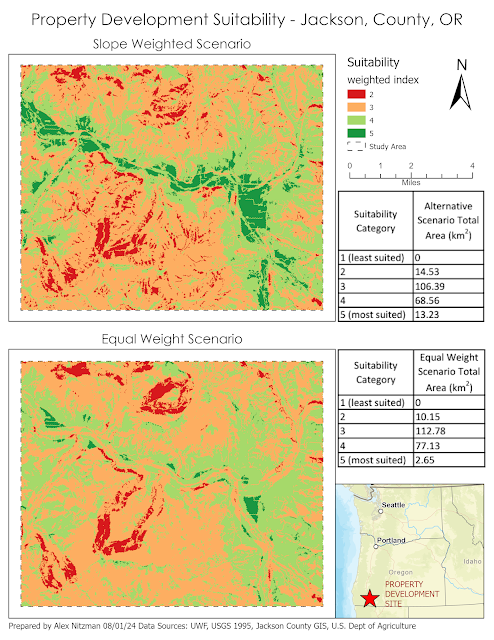
The final scenario for the lab of GIS Applications Module 6 is to determine a potential protected corridor linking two areas of black bear habitat in Arizona's Coronado National Forest. Data provided included the extent of the two existing areas of known black bear habitat, a DEM, a raster of land cover and a feature class of roads in the study area. Parameters required for a protected corridor facilitating the safe transit of black bear included land use away from population and preferably with vegetation, mid level elevations and distances far from roadways.

Geoprocessing flow chart for Scenario 4

The initial geoprocessing in our Corridor Suitability Analysis reclassifies the DEM and landcover rasters into suitability rasters using predetermined scales. The development of a suitability raster for the roads feature class commenced with creating a multi-ring buffer feature class, and then converting the derived polygons into a suitability raster using the Reclassify tool.

Reviewing the previous scenarios on outputting buffers from a polyline, I also ran the Euclidean Distance tool on the roads feature class. The succeeding output raster was then Reclassified using the distance suitability values that rank higher proximities with lower values. The results mirrored those using the Multi-Ring Buffer tool:

The suitability raster for the distance to roads derived from the raster output from the Euclidean Distance tool.

With suitability raster files finalized for elevation, landcover and proximity to roads, we can proceed with the analysis using the Weighted Overlay tool. The objective is to generate a cost raster using the integer scale of 1 through 10, based upon the influence percentages of 60% for land cover, 20% for elevation and 20% for distance to roads.

The result shows the highest suitability score for mid level elevations representative of undeveloped forest land that mostly avoids roads. Low level elevations represented by urban areas, agriculture and barren land factor into low suitability areas:

Weighted Overlay raster with the values of 1-10 where lighter colors represent lower suitability scores

Utilizing the Weighted Overlay raster, a cost surface raster is generated by using the Raster Calculator geoprocessing tool. The cost surface values were obtained by inverting the suitability model so that higher habitat suitability values translated into lower travel costs:

Cost Surface raster where the darker colors represent higher costs

With the Cost Surface raster, the Corridor Suitability Analysis continues with the Cost Distance tool run on the two Coronado National Forest black bear habitat area feature classes. This outputs Cost Distance and Cost Distance Backlink Rasters.

The cost distance raster for the northeastern unit of Coronado N.F.

The cost distance raster for the southwestern unit of Coronado N.F.

Together the two cost distance rasters for Coronado National Forest are the parameters for the Corridor geoprocessing tool, which generates the Least-Path Corridor raster. The threshold value for determining the best corridors was subjective, so I went with percentages used in the previous scenario, where the minimum destination cost value multiplied by 1.05 represented the optimal corridor. Chose a color scheme based upon the ColorBrewer web site.

The Least-Path Corridor for a protected Black Bear Corridor between Coronado National Forest units

Least-Cost Path and Corridor Analysis with GIS

The second half of Module 6 for GIS Applications conducts Least-Cost Path and Corridor Analysis on two scenarios. The first continues working with the Jackson County, Oregon datasets from Scenario 2.

There are several ways that GIS measures distance. Euclidean, the simplest, represents travel across a straight line or "as the crow flies". Manhattan distance simulates navigating along a city street grid, where travel is restricted to either north-south and east-west directions. Network Analysis models travel in terms of time, where travel is restricted by a road network or transit infrastructure.

Least-Cost Path Analysis models travel across a surface. It determines the single best course, a polyline, that has the lowest cost for a given source and destination, which are represented by points. This can be described as the routing over a landscape that is not restricted by road networks. 

The course through the landscape is modeled as a cost. More specifically each cell in a cost raster has a value which represents the cost of traveling through it.

Typical cost factors are slope and land cover. A cost surface can vary from just a single factor to a combination of them. Even if multiple factors are considered, the analysis only uses a single cost raster.

Least-Cost Path Analysis can be expanded to Corridor Analysis. Instead of resulting in a single base solution represented by a polyline, corridor analysis produces multiple solutions, representing a zone where costs are close to the least cost. The corridor width uses is somewhat subjective. It is controlled by deciding what range of cost to consider. Values of a few percentage points above the lowest cost to as much as 10% above the lowest cost are common.

Scenario 3 uses least-cost path analysis on an area of land in the planning for a potential pipeline. Cost factors include elevation, proximity to rivers and potential crossings of waterways. Datasets used for these cost factors include a DEM, a rivers feature class and feature classes determining the source and destination of the proposed pipeline. Analysis proceeds focusing on each cost factor individually.

Geoprocessing flowchart for least-cost path analysis factoring solely on slope

Focusing first on the DEM, the raster is converted to a slope raster, and subsequently reclassified using a cost factor range of eight values. The next analysis step utilizes the Cost Distance geoprocessing tool. Using an iterative algorithm, a cost distance raster is generated that represents the accumulated cost to reach a given cell from the source location point.

A cost backlink raster is also created, which traces back how to reach a given cell from the source. This reveals the actual path utilized to obtain the lowest cost. The actual cell values of the backlink raster represent either cardinal directions or the intercardinal point (NE, NW, etc.) instead of cost. The combination of the two output rasters contain every least cost path solution from the single source to all cells within the study area.

Cost Distance Raster - Values represent the cost of traveling through a cell

Cost Distance Backlink Raster - Values correspond with compass directions

The final step of least cost path analysis obtains the least cost path from the source to one or more destinations. The result of the Cost Path geoprocessing tool, this consists of a single polyline representing the lowest accumulated cost.

The result of Least-Cost Path Analysis solely on slope

Continuing our analysis of a proposed pipeline in Jackson County, Oregon, we factor in river crossings as a cost factor.

Geoprocessing flowchart for least-cost path analysis factoring in both slope and river crossings

The result of factoring in river crossings to the cost analysis reduces potential crossings to five from the 16 when factoring in slopes alone:

Furthering our analysis, we change from factoring in river crossings to instead factor in the distance to waterways. Using a multiple ring buffer, cost factors are set high for areas within 100 meters of hydrology and moderate for areas within 500 meters. Distances beyond 500 meters from a waterway are zero, reflecting no cost.

Geoprocessing flowchart for least-cost path analysis factoring slope and proximity to waterways

As the cost factor criterion for the least-cost path analysis is adjusted to better compensate natural factors, the least cost path adjusts accordingly:

The final analysis for third scenario looks at Least-Cost Path Corridor Analysis, which not only includes the least-cost path, but also a multiple of other least-cost alternatives within a corridor determined on a case-by-case basis.

Geoprocessing flowchart for least-cost path corridor analysis

The geoprocessing to develop the least-cost path corridor utilizes the previously generated cost raster factoring in the proximity to waterways and slope. Instead of using the source point as the feature source data, the Cost Distance tool is based off the destination point feature class.

Together the two cost distance rasters, one based off the "destination" feature class and the other off the "source" feature class, are input into the Corridor geoprocessing tool. This outputs the Least-Path Corridor raster, which areas of least-cost paths symbolized based upon a percentage from the minimum cost value:

Suitability Modeling with GIS

Module 6 for GIS Applications includes four scenarios conducting Suitability and Least-Cost Path and Corridor analysis. Suitability Modeling identifies the most suitable locations based upon a set of criteria. Corridor analysis compiles an array of all the least-cost paths solutions from a single source to all cells within a study area.

For a given scenario, suitability modeling commences with identifying criteria that defines the most suitable locations. Parameters specifying such criteria could include aspects such as percent grade, distance from roads or schools, elevation, etc.

Each criteria next needs to be translated into a map, such as a DEM for elevation. Maps for each criteria are then combined in a meaningful way. Often Boolean logic is applied to criteria maps where suitability is assigned the value of true and non suitable is false. Boolean suitability modeling overlays maps for all criteria and then determines where all criterion is met. The result is a map showing areas suitable versus not suitable.

Another evaluation system in suitability modeling use Scores or Ratings. This scenario expresses criterion as a map showing a range of values from very low suitability to very high, with intervening values in between. Suitability is expressed as a dimensionless score, often by using Map Algebra on associated rasters.

Scenario 1 for lab 6 analyzes a study area in Jackson County, Oregon for the establishment of a conservation area for mountain lions. Four sets of criterion area are specified. Suitable areas must have slopes exceeding 9 degrees, be covered by forest, be located within 2,500 feet of a river and more than 2,500 feet from highways. 

Flowchart outlining input data and geoprocessing steps.

Working with a raster of landcover, a DEM and polyline feature classes for rivers and highways, we implement Boolean Suitability modeling in Vector. The DEM raster is converted to a slope raster, so that it can be reclassified into a Boolean raster where slopes above 9 feet are assigned the value of 1 (true) and those below 0 (false). The landcover raster is simply reclassified where cells assigned to the forest land use class are true in the Boolean.

Buffers were created on the river and highway feature classes, where areas within 2,500 feet of the river are true for suitability and areas within 2,500 feet of the highway are false for suitability. Once the respective rasters are converted to polygons and the buffer feature classes clipped to the study area, a criteria union is generated using geoprocessing. The suitability is deduced based upon the Boolean values of that feature class and selected by a SQL query to output the final suitability selection.

We repeat this process, but utilizing Boolean Suitability in Raster. Using the Euclidean Distance tool in ArcGIS Pro, buffers for the river and highway feature classes were output as raster files where suitability is assigned the value of 1 for true and 0 for false. Utilized the previously created Boolean rasters for slope and landcover.

Obtaining the suitable selection raster with the four rasters utilizes the Raster Calculator geoprocessing tool. Since the value of 1 is true for suitability in the four rasters, simply adding the cell values for all result in a range of 0 to 4, where 4 equates to fully suitable. The final output was a Boolean where 4 was reclassified as 1 and all other values were assigned NODATA.

Scenario 2 determines the percentage of a land area suitable for development in Jackson County, Oregon. The suitability criteria ranks land areas comprising meadows or agricultural areas as most optimal. Additional criterion includes soil type, slopes of less than 2 degrees, a 1,000 foot buffer from waterways and a location within 1,320 feet of existing roads. Input datasets consist of rasters for elevation and landcover, and feature classes for rivers, roads and soils.

Flowchart of the geoprocessing for Scenario 2

With all five criteria translated into respective maps, we proceed with combining them into a final result. However with Scenario 2, the Weighted Overlay geoprocessing tool is implemented. This tool utilizes a percentage influence on each input raster corresponding to the raster's significance to the criterion. The percentages of each raster input must total 100 and all rasters must be integer-based.

Cell values of each raster are multiplied by their percentage influence and the results compiled in the generation of an output raster. The first scenario evaluated for lab 6 includes an equal weight scenario, where the 5 raster files have the same percentage influence (20%). The second scenario assigned heavier weight to slope (40%) while retaining 20% influence to land cover and soils criterion, and decreasing the percentage influence of road and river criterion to 10%. The final comparison between the two scenarios:

Opted to symbolize the output rasters using a diverging color scheme from ColorBrewer.